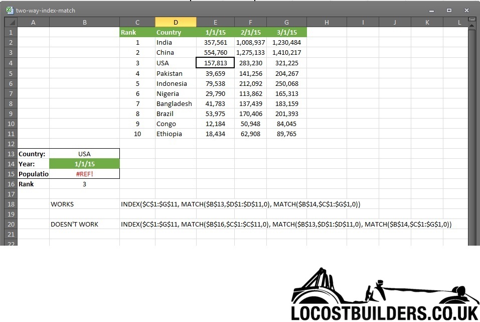
Hi I’m having a bad day with excel and thanks to the kids keeping me awake for the last 4 nights I'm really not in the humour for fighting computers.

I'm trying to sort out a formula for building a much larger spreadsheet I need at work but just cannot get it sorted out.

All I want to do is lookup 2 columns and 1 row along the top which is a date, I can get it to work for 1 row and 1 column but not 2 columns, excel is so hopeless for suggesting what is wrong. If I put USA, 1/1/15 & rank 3 I want it to read 157,813 in B15 not #REF!

I have put the working and not working formulas down at the bottom so you can see what I've been doing.

Help would be appreciated, thanks in advance



[Edited on 20/10/15 by Mr Whippy]

The easiest thing to do is concatenate column c and d together to give you 3USA in another column e for instance and search in a single column for that


=INDEX(C1:H11, MATCH(B16&B13,E1:E11,0),MATCH(B14,C1:H1,0))

Cheers
David

quote:

---

Originally posted by Minicooper
The easiest thing to do is concatenate column c and d together to give you 3USA in another column e for instance and search in a single column for that


=INDEX(C1:H11, MATCH(B16&B13,E1:E11,0),MATCH(B14,C1:H1,0))

Cheers
David

---

The code in "Doesn't work" doesn't work because the fourth argument to the INDEX function is only used to select which range to use when multiple ranges have been specified in the first argument. Since you have only specified a single range in the first argument, the function is returning an error.

Sorry if I'm being thick, but I don't really understand what you are trying to do. How can you reference a two dimensional table with three dimensions (Rank, Date and Country)? Surely rank is something you would calculate for a specific country according to it's population on a particular date? It doesn't make sense to me why you have the Rank as a column with fixed numbers in your dataset.

If you want to calculate rank given a country and date, then the following should do the trick:

B15 =INDEX($C$2:$G$11,MATCH($B$13,$D$2:$D$11,0),MATCH($B$14,$C$1:$G$1,0))
B16 =RANK.EQ($B$15,OFFSET($E$2:$E$11,0,MATCH($B$14,$E$1:$G$1,0)-1))