Mr Whippy
|
 posted on 10/9/14 at 11:09 AM posted on 10/9/14 at 11:09 AM |

|
|
Excel SumIFs help...

Hi,
Excel help needed again, been a long night with the wee one and yet again next day its formula time
feck no cup of coffee is that powerful!
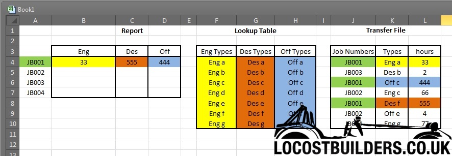
What Im trying to do is get a SUMIFS to work so that it looks up the job number shown in say A7 over in the Transfer file table and sums the hours
where the Type also matches the range in the Lookup table.
Thanks in advance   
|
|
|
|
|
MikeRJ
|
| posted on 10/9/14 at 11:38 AM |

|
|
I don't quite understand how the Types field is supposed to work in the "Transfer File" table?
e.g. given the current data, if you changed K4 from 'Eng a' to 'Eng b', would the hours change?
|
|
|
Mr Whippy
|
| posted on 10/9/14 at 11:46 AM |

|
|
no the hours in B4 would be the same
Maybe I'm not doing a good job of explaining it...
For JB001, any type in K4 - K10 that has a value which matches any of those listed in the range F4 - F10 should be totalled in the ENG cell B4. So
I'm matching Job number and types but the valid types are shown in the Look up table for Eng, Des, Off
Thanks, Scott
|
|
|
Ivan
|
| posted on 10/9/14 at 12:04 PM |

|
|
I don't think it can be done without some preliminary steps or If/Then type nested formulas.
|
|
|
pekwah1
|
| posted on 10/9/14 at 12:30 PM |

|
|
can be done.
Try this:
=sumifs(L:L, J:J, A4)
L:L gives you the SUM RANGE so where it will count from
J:J gives you the CRITERIA RANGE so the column it will validate
A4 is the cell we are using at the criteria
Should do what you want!
--EDIT--
Just re-read what you are after, this won't do it
[Edited on 10/9/14 by pekwah1]
|
|
|
pekwah1
|
| posted on 10/9/14 at 12:52 PM |

|
|
Ok, this might give you something to go on....
=SUMIFS(L:L, J:J,A4,F:F,"Eng*"
You will have to be explicit with the "Eng" or "Off" etc that you want to search on, so it isn't actually cross
referencing the other table.
but you can use the * wildcard so that it would match Eng a, eng b etc.
Any good?
|
|
|
pekwah1
|
| posted on 10/9/14 at 01:31 PM |

|
|
Clearly i've got nothing better to do with my time....
i have managed to do it, but you might need to add some extra columns onto the third table as below:

Basically we are validating in the yellow columns if the code exists in the second table and returning a 1 if it does.
We can then use that criteria in the first column to count the number of hours per department.
obviously you can just hide the extra columns or make them white text etc.
Formulas are (can be copied across cells):
Cell B4 =SUMIFS($L:$L,$J:$J,$A4,M:M, 1)
Cell M4 =COUNTIF(F:F, $K4)
Hope this helps!
|
|
|
Mr Whippy
|
| posted on 10/9/14 at 02:11 PM |

|
|
Fab thanks very much 
I'll have a go with that and see if I can use it, I've spent almost all day on this spreadsheet and I'm burnt out, it's not
even for me! but I agreed to help the costy ask he has no idea at all about excel
Cheers for your time 
|
|
|
gingerprince
|
| posted on 10/9/14 at 06:26 PM |

|
|
If you can change the format of your lookup slightly then a Pivot table will be much easier. e.g.

Relayout the lookup as per column A and B. Use VLOOKUP to calculate an extra field in column G : =VLOOKUP(E2,$A$1:$B$22,2,0)
Then simply drop a basic pivot table based on D:G, choosing Job No vs Class and summing Hours.
Example linked here: -
https://dl.dropboxusercontent.com/u/7785198/excelsheet.xls
It's an old excel format but you should be able to open it in any version.
This of course assumes you have the liberty of reformating your lookup 
If you can't reformat, then you could do a nested IF/VLOOKUP to generate column G then proceed with the Pivot again.
|
|
|
gingerprince
|
| posted on 10/9/14 at 07:08 PM |

|
|
However if you want to avoid pivots then you can do it with a single helper field. Using your cell references example, set M4 to this formula and
drag down: -
=CONCATENATE(J4,":",IF(NOT(ISERROR(VLOOKUP(K4,$F$4:$F$10,1,0))),"Eng",IF(NOT(ISERROR(VLOOKUP(K4,$G$4:$G$10,1,0))),"Des&
quot;,IF(NOT(ISERROR(VLOOKUP(K4,$H$4:$H$10,1,0))),"Off","Invalid Value" ))) )))
That'll create a helper that looks like this: -
JB001:Eng
JB003 es es
JB001:Off
JB002:Eng
JB001 es es
JB002:Off
JB004:Eng
Then in B4 use =SUMIF($M$4:$M$10,CONCATENATE($A4,":Eng" ,$L$4:$L$10) ,$L$4:$L$10)
Then in C4 use =SUMIF($M$4:$M$10,CONCATENATE($A4," es" es" ,$L$4:$L$10) ,$L$4:$L$10)
Then in D4 use =SUMIF($M$4:$M$10,CONCATENATE($A4,":Off" ,$L$4:$L$10) ,$L$4:$L$10)
Drag them down.
These will compare column A concatenated with ":Eng" " es" and ":Off" respectively and add them up. es" and ":Off" respectively and add them up.
I would recommend using Pivot tables though. If you don't know how to use them, put some time in and learn they can save a lot of effort once
you're used to them.
Example sheet here
https://dl.dropboxusercontent.com/u/7785198/excelsheet2.xls
[Edited on 10/9/14 by gingerprince]
|
|
|


